NLP for learners-Training and prediction with keras and LSTM
In the Extract the text of the article from the URL, We extracted the text from VOA Learning English. This time, we use it for deep learning.
TensorFlow and Keras
To perform deep learning, you need to install TensorFlow and Keras.
Deep Learning Procedures
First, we load the text file to be trained and create a dictionary. Next, convert the characters to vectors and create the input values and answers for the model. When the data is ready for training, the model is built and trained. Finally, save the trained model.
In this case, we are going to build a model that predicts the next word based on the five words.
Loading text
with io.open('articles.txt', encoding='utf-8') as f:
    text = f.read().splitlines()
Reads the text file articles.txt. It is 318KB in size.
texts = text.replace('eos', 'eos\n').splitlines()
Add a line break character to the end-of-sentence sign eos and store the text line by line in the list texts with .spilitlines().
Creating a dictionary
Tokenizer makes it easy to pre-process text. The Tokenizer is included in Keras.
In deep learning, characters cannot be used as data as they are. We can only work with numbers. So, we create a dictionary and replace words with numbers.
tokenizer = Tokenizer()Create an object tokenizer. You can imagine that a machine is created to automatically process the text, and its name is tokenizer.
tokenizer.fit_on_texts(texts).fit_on_texts() gives the text to the tokenizer.
char_indices = tokenizer.word_index.word_index creates a list of dictionary types and stores it in list char_indices.
char_indices = {'the': 1, 'in': 2, 'to': 3, 'and': 4, 'of': 5, ... , 'jr': 390, 'editor': 391}A number has been assigned to the words used in the text. The list is ordered by the frequency of the words. The total number of words is 6950.
The tokenizer also automatically converts words to lowercase and removes marks such as double quotation and colons.
indices_char = dict([(value, key) for (key, value) in char_indices.items()])Creates a reverse dictionary and stores it in indices_char. dict() creates a list of dictionary types.
indices_char = {1: 'the', 2: 'in', 3: 'to', 4: 'and', 5: 'of', .... , 390: 'jr', 391: 'editor'}The result of the prediction is returned in a number representing the word. Then, using a reverse dictionary, the number is converted back to a word and the result is checked.
Vectorization of words
pre_vec = tokenizer.texts_to_sequences(texts).texts_to_sequences() vectorizes the words and stores them in the list pre_vec
pre_vec =
[[1, 30, 68, 14, 69, 125, 70, 5, 126, 2, 37, 3, 9, 2, 38, 3, 127, 1, 128, 5, 12, 129, 1, 130, 131],
 [1, 10, 71, 13, 132, 3, 133, 45, 18, 20],
 [1, 20, 46, 47, 6, 2, 134, 21, 1, 14, 4, 135, 21, 1, 136, 137],

 ......

]
A word is represented by a single value. This is the same as saying that the values are one-dimensional vectors. But we might not call it a vector.
In fact, a word can have more than one value. For example, if we represent a word as (13,87,25), this would be a three-dimensional vector, sometimes called a third-order tensor.
The value of a one-dimensional vector has little meaning. All we can learn from its value is the frequency of the word’s appearance.
Increasing the dimension of the vectors can give more information to the words and allow for more advanced learning.
texts_vec = []
for line in range(len(pre_vec)):
    if len(pre_vec[line]) > 9:
        texts_vec.append(pre_vec[line])
len(pre_vec) is the number of lines of text and len(pre_vec[line]) is the number of words in line.
If there are more than 10 words, the transformed vector is stored in the list texts_vec and the short lines are cut.
In this case, each line must have at least six words, since the next word is predicted based on the previous five words.
Prepare the data set
seq_length = 5In this case, we will predict the next word based on the previous five words. This is represented by seq_length.
The input values take the form of (batch size, time step, input dimension).
The five-value set is a time step. The time steps are created by shifting the words one by one, and the total is the batch size. The answer is then one word following each time step. The input dimension is the dimension of the word vector. In this case, the dimension is 1.
Create a time step.
for line in range(len(texts_vec)):
    for i in range(len(texts_vec[line])-5):
line is the line number and i is the position of a word in the line, where i is up to five less than the number of words in each line.
        x.append(texts_vec[line][i:i+5])
        y.append(texts_vec[line][i+5])
x is the input value given to the model. [i:i+5] represents the range of the list. For example, a value of i of 0 means from 0 to 4, not from 0 to 5.
The iterative process begins with line=0 and i=0. .append() is used to add the values from texts_vec[0][0] to texts_vec[0][4] to list x. Then i=1, and the values from texts_vec[0][1] to texts[0][5] are added. Thus, the five pairs of values are extracted one by one.
x =
[[1, 30, 68, 14, 69],
 [30, 68, 14, 69, 125],
 [68, 14, 69, 125, 70],

 ......

]
y is the answer. text_vec[0][5] is added when line=0 and i=0.
y =
[125,
 70,
 5

 ......

]
y means the value that should be predicted. The model is trained to output the same value as y for an input value given by x. The model is trained to return the same value as y. Untrained models return random values, but as the training progresses, they have a high probability of outputting the same value as y.
x = np.reshape(x,(len(x),seq_length,1))np.reshape() changes the shape of the list. The input values given to the model must be three-dimensional vectors.
x =
[[[  1]
  [ 30]
  [ 68]
  [ 14]
  [ 69]]

 [[ 30]
  [ 68]
  [ 14]
  [ 69]
  [125]]

 [[ 68]
  [ 14]
  [ 69]
  [125]
  [ 70]]

 ......

]
Alternatively, we can prepare an empty three-dimensional list and store the values one by one. However, np.reshape() is faster.
Creating a one-hot list
y = np_utils.to_categorical(y, len(char_indices))np_utils.to_categorical() converts a list into a one-hot format.
For example, if all words are represented by a value between 0 and 4, each value is represented in one-hot form as
0 ---> [1,0,0,0,0]
1 ---> [0,1,0,0,0]
2 ---> [0,0,1,0,0]
3 ---> [0,0,0,1,0]
4 ---> [0,0,0,0,1]
In this case, the total number of words is 6950, but the model returns the probability for each word as the output value.
result =
[[5.21713228e-10 3.66212561e-07 1.54906775e-05 6.71785965e-05
  2.40655282e-07 3.59350683e-09 4.46252926e-07 4.50365405e-07
  2.32367552e-06 3.77001937e-11 2.18020944e-08 2.20234284e-07
  2.27694059e-07 1.82693594e-08 1.24455757e-09 1.38001795e-07

  ......

]]
We take the most probable one from the list as the prediction result.
The model compares the answer y with the result and modifies the model so that the prediction approaches the answer.
Building the Model
model = Sequential()Build an object model, which can be imagined as a machine learning a natural language, giving the model input and receiving output, with Sequential() indicating that the model is chained together.
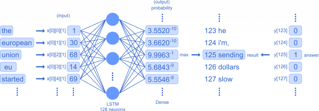
This is an overview of the training process. Each word is converted to a vector and stored in x. The five word pairs (time steps) are fed to the LSTM one by one and then aggregated into the Dense layer, which outputs the probability of each word in the dictionary and determines the highest probability as the prediction. It also calculates the error between the output values and the answer y that was prepared in advance, and corrects the error so that the gap between the output values and the answer y is small by going back through the network.
model.add(LSTM(128, input_shape=(seq_length, 1)))Add an LSTM layer to the model; the LSTM is the actual layer for the training. We install 128 neurons.
input_shape=(seq_length, 1) describes the shape of the input value in each neuron. seq_length=5, so each neuron is given data with a size of (5,1).
model.add(Dense(y.shape[1], activation='softmax'))Aggregates the output of the LSTM into a Dense layer, which outputs the probability of each word. y.shape[1] is the total number of words in the dictionary.
activation='softmax' indicates that the softmax function is used as the activation function, and the softmax function calculates the probability for each word.
optimizer = Adam(lr=0.01)Specify Adam as an optimization function. The optimization function is used to correct for errors between the output value and the answer.
lr=0.01 is the learning rate. If we increase the value of learning rate, the problem occurs that while the learning speed becomes faster, the accuracy does not increase. On the other hand, if we reduce the value of the learning rate, the problem occurs that while the accuracy improves, the learning speed slows down.
model.compile(loss='categorical_crossentropy', optimizer=optimizer, metrics=['accuracy'])loss='categorical_crossentropy' indicates the use of cross entropy error as the loss function. The loss function is a measure of the error between the result and the answer. The model uses the value of the loss function to modify the network in such a way that the value of the loss function is reduced.
metrics=['accuracy'] represents the use of precision as a way to evaluate the model.
Learning Execution
model.fit(x, y, epochs=100, verbose=1)model.fit() gives the model an input value x and an answer y to train.
Training is done in epochs, and the more epochs you have, the more accurate the training becomes. This time, we will train 100 epochs.
verbose specifies a way to display the progress status; if verbose=0, the progress status is not displayed.
.fit() will produce the following output
Epoch 1/100
37858/37858 [==============================] - 7s 193us/step - loss: 6.9415 - accuracy: 0.0759

......

Epoch 100/100
37858/37858 [==============================] - 6s 171us/step - loss: 4.4052 - accuracy: 0.1814
The batch size is 37858, which means that there are 37858 word pairs (time steps). Training results show that the model is 18.14 percent accurate. This is not a good result.
Normalization of input values
x = x / float(len(char_indices))
To improve the result, the input values are normalized. float() converts an integer to floating point. The maximum input value is equal to the size of the dictionary, and if you divide the value by the size of the dictionary, x will be a fractional number between 0 and 1. This is called normalization.
The model outputs the probability for each word as a value between 0 and 1. In this case, the closer the input and output scales are, the more efficient the learning is.
Epoch 100/100
37858/37858 [==============================] - 6s 166us/step - loss: 1.7827 - accuracy: 0.5174
Accuracy improved to 51.74 percent.
Saving the model
model.save('model_voa.h5')Save the trained model in the file model_voa.h5. You can load the saved model and make predictions later.
np.save('char_indices_voa', char_indices)
np.save('indices_char_voa', indices_char)
np.save('x_voa.npy', x)
np.save('y_voa.npy', y)
Save dictionaries and datasets to a file. We’ ll need these files later on when we make a prediction.
Here is the whole code.
import numpy as np
import sys
import io
import os
os.environ['TF_CPP_MIN_LOG_LEVEL']='2'
from keras.models import Sequential
from keras.layers import Dense
from keras.layers import LSTM
from keras.optimizers import Adam
from keras.utils import np_utils
from keras.preprocessing.text import Tokenizer
#read the text
with io.open('articles.txt', encoding='utf-8') as f:
    text = f.read()
texts = text.replace('eos', 'eos\n').splitlines()
#make the dictionary
tokenizer = Tokenizer()
tokenizer.fit_on_texts(texts)
char_indices = tokenizer.word_index
#make the inverted dictionary
indices_char = dict([(value, key) for (key, value) in char_indices.items()])
np.save('char_indices_voa', char_indices)
np.save('indices_char_voa', indices_char)
#vectorization and short lines cut
pre_vec = tokenizer.texts_to_sequences(texts)
texts_vec = []
for line in range(len(pre_vec)):
    if len(pre_vec[line]) > 9:
        texts_vec.append(pre_vec[line])
#make dataset
print('make the dataset....')
seq_length = 5
chars = []
x = []
y = []
for line in range(len(texts_vec)):
    for i in range(len(texts_vec[line])-5):
        x.append(texts_vec[line][i:i+5])
        y.append(texts_vec[line][i+5])
np.save('x_voa.npy', x)
np.save('y_voa.npy', y)
x = np.reshape(x,(len(x),seq_length,1))
x = x / float(len(char_indices))
#convert y into one-hot
y = np_utils.to_categorical(y, len(char_indices)+1)
#build the model
print('build the model....')
model = Sequential()
model.add(LSTM(128, input_shape=(seq_length, 1)))
model.add(Dense(y.shape[1], activation='softmax'))
optimizer = Adam(lr=0.01)
model.compile(loss='categorical_crossentropy', optimizer=optimizer, metrics=['accuracy'])
#learning
model.fit(x, y, epochs=100, verbose=1)
#save the model
model.save('model_voa.h5')
Predict the results
Check whether the model we have built is actually predictive or not.
with io.open('articles.txt', encoding='utf-8') as f:
    text = f.read().splitlines()
texts = text.replace('eos', 'eos\n').splitlines()
char_indices = np.load('char_indices_voa.npy', allow_pickle=True).tolist()
indices_char = np.load('indices_char_voa.npy', allow_pickle=True).tolist()
x = np.load('x_voa.npy', allow_pickle=True)
y = np.load('y_voa.npy', allow_pickle=True)
Load stored text, dictionaries and datasets.
model = load_model('model_voa.h5')Loads a saved model.
for pattern in range(5):An iterative process makes five predictions.
    for i in range(seq_length):
        x_pred.append(x[pattern][i])
        chars.append(indices_char[x[pattern][i]])
.append() adds the values created in the dataset to the list x_pred.
It also uses a reversed dictionary to convert the value back to a word and adds it to the list chars.
    x_pred = np.reshape(x_pred,(1, seq_length, 1))
    x_pred = x_pred / float(len(char_indices))
As in training, change the shape of the input values (batch size, time step, and input order).
prediction = model.predict(x_pred, verbose=0)
Give x_pred to model.predict() and make a prediction. The probability of each word is stored in the list prediction.
index = np.argmax(prediction)
np.argmax() finds the maximum value from a list of values. It stores the maximum value in index.
result = indices_char[index]
Reverse lookup dictionary is used to convert the value back to a word and store it in result.
char = ' '.join(chars)
Concatenates list chars into a single string char.
    print(char)
    print('  answer:'+str(indices_char[y[pattern]]))
    print('  prediction:'+str(result))
Execute the code and display the result.
the european union eu started
  answer:sending
  prediction:sending
european union eu started sending
  answer:millions
  prediction:millions
union eu started sending millions
  answer:of
  prediction:of
eu started sending millions of
  answer:dollars
  prediction:dollars
started sending millions of dollars
  answer:in
  prediction:eos
We can see that the output and the answer are consistent and predicted correctly with a high probability.
SNSでシェア